A few days ago, I read the book "Make Your Own Neural Network" by Tariq Rashid. It is a practical introduction to neural networks.
The book describes how to build a basic feedforward neural network with forward propagation and backpropagation. If you already know the basics of neural networks, you will probably not learn anything new from it. For me, as a beginner, it was a very approachable introduction.
In the first part of the book, the author explains the core ideas behind neural networks. In the second part, he presents an example based on the MNIST dataset. MNIST is a large collection of handwritten digits that is widely used for training and testing machine learning models. It contains 60,000 training images and 10,000 test images. Each image has a size of 28 x 28 pixels and depicts a digit between 0 and 9. Using separate training and test sets is a standard way to evaluate how well a model generalizes and to reduce the risk of overfitting.
Most machine learning tutorials and frameworks still assume Python, so all the examples in Tariq's book are written in that language. The algorithms in the book do not depend on a machine learning framework, though, so they translate quite well to other languages. To experiment with the ideas, I wrote one implementation in Java and one in JavaScript. Because the example performs many matrix calculations, both projects use external libraries for matrix support.
Here's an overview of the neural network I'm using in the following example.

The network consists of three layers: input, hidden, and output layer. The input layer contains 784 nodes. One node represents one pixel of the scanned image (28 x 28 = 784).
The hidden layer contains 200 nodes and the output layer contains 10 nodes. The purpose of this neural network is to detect which digit the scanned image represents, so it needs 10 output nodes. If we feed an image of the digit 1 into the network, the ideal output is [0, 1, 0, 0, 0, 0, 0, 0, 0, 0].
Each node between the input and hidden layers, and between the hidden and output layers, is connected. Each connection has a weight, and these weights are what change during training.
During the learning process, each image runs through the following steps:
Forward propagation
- Each pixel of the image is assigned to an input node.
- For each connection between the input and hidden layer, multiply the value of the input node by the weight and apply an activation function. This example uses sigmoid. The resulting values become the hidden layer output.
- Repeat the same process for each connection between the hidden and output layer.
Backpropagation
- Compare the values in the output layer with the target values. For instance, if we feed the scanned image of a 7, we want
[0, 0, 0, 0, 0, 0, 0, 1, 0, 0]as the output. - To learn, the network calculates how far the output is from the target values and adjusts the weights accordingly. The correction is applied to both sets of connections: output to hidden and hidden to input.
After step 5, the application feeds the next image into the network and starts again with step 1. It does that for all 60,000 training images and repeats the full process 10 times, one pass per epoch.
This is how a neural network learns: data is fed into it, the output results are compared with the expected results, and the difference is minimized by adjusting the weights between the nodes.
I will not go into more detail about the algorithms here. Tariq explains them well in the book, and this post focuses on the implementation rather than the theory.
There is also a lot of free material online. A good companion resource for this example is Google's Neural Networks module in Machine Learning Crash Course, which walks through the same building blocks from a current perspective.
Example 
The example consists of two applications: a Java application for training the network and a TypeScript browser application built with Angular and Ionic for using the pre-trained model to detect digits drawn into a canvas. The detection process does not require a back-end server and runs entirely in the browser.
You can find the complete source code on GitHub: https://github.com/ralscha/blog/tree/master/mnist
Java 
The Java application reads the MNIST dataset and trains the network.
The MNIST dataset can be downloaded from TensorFlow's public mirror:
- train-images-idx3-ubyte.gz
- train-labels-idx1-ubyte.gz
- t10k-images-idx3-ubyte.gz
- t10k-labels-idx1-ubyte.gz
The application expects all four files to be present in the project's root directory:
- train-images-idx3-ubyte.gz
- train-labels-idx1-ubyte.gz
- t10k-images-idx3-ubyte.gz
- t10k-labels-idx1-ubyte.gz
The train files contain the 60,000 training images, and the t10k files contain the 10,000 test images.
The images files contain the pixel data, and the label files contain the corresponding digit for each image. A label is a number between 0 and 9.
As mentioned before, many of the calculations can be quite efficiently handled with matrix calculations. Java does not have built-in support for matrices; therefore, I added the Apache commons-math library to the project.
    <dependency>
      <groupId>org.apache.commons</groupId>
      <artifactId>commons-math3</artifactId>
      <version>3.6.1</version>
    </dependency>
The application first creates the matrices for the connections between the input and hidden layers and between the hidden and output layers, and then assigns a random weight to each connection.
    wInputHidden = createRealMatrix(HIDDEN_NODES, INPUT_NODES);
    wHiddenOutput = createRealMatrix(OUTPUT_NODES, HIDDEN_NODES);
    wInputHidden = initRandom(wInputHidden, Math.pow(INPUT_NODES, -0.5));
    wHiddenOutput = initRandom(wHiddenOutput, Math.pow(HIDDEN_NODES, -0.5));
Next, the application reads the labels and image data from the MNIST files. For each image, it creates two additional versions: one rotated 10 degrees clockwise and one rotated 10 degrees counterclockwise. This data augmentation step helps improve the model's accuracy.
    int[] labels = MnistReader.getLabels(Paths.get("./train-labels-idx1-ubyte.gz"));
    List<int[][]> images = MnistReader
        .getImages(Paths.get("./train-images-idx3-ubyte.gz"));

    double[][] scaledImages = new double[images.size()][];
    for (int i = 0; i < images.size(); i++) {
      scaledImages[i] = scale(Util.flat(images.get(i)));
    }

    double[][] rotatedClockwiseScaledImages = new double[images.size()][];
    for (int i = 0; i < images.size(); i++) {
      rotatedClockwiseScaledImages[i] = scale(Util.flat(rotate(images.get(i), 10)));
    }

    double[][] rotatedCounterclockwiseScaledImages = new double[images.size()][];
    for (int i = 0; i < images.size(); i++) {
      rotatedCounterclockwiseScaledImages[i] = scale(Util.flat(rotate(images.get(i), -10)));
Then it feeds all three images into the neural network. The application multiplies the input values by the weights, applies the sigmoid function, and repeats the same calculation from the hidden layer to the output layer.
  private static void train(RealMatrix inputs, RealMatrix targets) {
    // forward
    RealMatrix hiddenInputs = wInputHidden.multiply(inputs);
    RealMatrix hiddenOutputs = scalar(hiddenInputs, Util::sigmoid);

    RealMatrix finalInputs = wHiddenOutput.multiply(hiddenOutputs);
    RealMatrix finalOutputs = scalar(finalInputs, Util::sigmoid);
During backpropagation, the application calculates the difference between the predicted values and the target values and applies correction values to the weights between the output and hidden layers and between the hidden and input layers.
    // back
    RealMatrix outputErrors = targets.subtract(finalOutputs);
    RealMatrix t1 = multiplyElements(outputErrors, finalOutputs);
    RealMatrix t2 = multiplyElements(t1, scalar(finalOutputs, in -> 1.0 - in));
    RealMatrix t3 = t2.multiply(hiddenOutputs.transpose());
    wHiddenOutput = wHiddenOutput.add(scalar(t3, in -> LEARNING_RATE * in));

    RealMatrix hiddenErrors = wHiddenOutput.transpose().multiply(outputErrors);
    t1 = multiplyElements(hiddenErrors, hiddenOutputs);
    t2 = multiplyElements(t1, scalar(hiddenOutputs, in -> 1.0 - in));
    t3 = t2.multiply(inputs.transpose());
    wInputHidden = wInputHidden.add(scalar(t3, in -> LEARNING_RATE * in));
After running all scanned images through the learning process, the application writes the weights into two files.
    writeJson(wInputHidden, "./weights-input-hidden.json");
    writeJson(wHiddenOutput, "./weights-hidden-output.json");
This is the "knowledge" of the neural network: the weights between the layers. In this basic example, the topology is hardcoded, so we only need to persist the weights for the 784 input, 200 hidden, and 10 output nodes.
The JavaScript application reads these two files and uses the pre-trained model to detect user-generated input.
After training, the program runs the 10,000 test images through the network and calculates the accuracy. In my tests, it reached about 97.6%, which is a solid result for such a small implementation.
JavaScript 
The web application is written in TypeScript with Angular and Ionic. It consists of a single page with a canvas element. The user draws a digit with a finger or a mouse, and the application uses the pre-trained neural network to detect it.
Like in Java, JavaScript does not have built-in support for matrix calculations; hence, I added the mathjs library to the project.
npm install mathjs
The two weight files from the Java application live in the assets folder, so the browser can fetch them directly at startup.
  private readonly weightsLoaded: Promise<void>;
  private weightsInputHidden!: number[][];
  private weightsHiddenOutput!: number[][];

  constructor() {
    this.weightsLoaded = this.loadWeights();
  }

  private async loadWeights(): Promise<void> {
    const [weightsInputHidden, weightsHiddenOutput] = await Promise.all([
      fetch('assets/weights-input-hidden.json').then(
        (response) => response.json() as Promise<number[][]>,
      ),
      fetch('assets/weights-hidden-output.json').then(
        (response) => response.json() as Promise<number[][]>,
      ),
    ]);

    this.weightsInputHidden = weightsInputHidden;
    this.weightsHiddenOutput = weightsHiddenOutput;
  }
Because the application uses a pre-trained model, it only has to implement forward propagation. The code works exactly like the Java version: multiply the input values by the weights, apply the sigmoid activation function, and repeat the calculation for the hidden-to-output connections.
  private forwardPropagation(imageData: number[]): number[] {
    const inputs: number[][] = [];
    for (const id of imageData) {
      inputs.push([id]);
    }

    const hiddenInputs = multiply(this.weightsInputHidden, inputs);
    const hiddenOutputs = hiddenInputs.map((row) => row.map((value) => this.sigmoid(value)));
    const finalInputs = multiply(this.weightsHiddenOutput, hiddenOutputs);
    return finalInputs.map((row) => row.map((value) => this.sigmoid(value))).flat();
  }
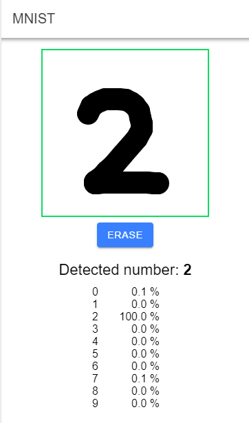
Each time the user finishes drawing a digit, the application scales the image down to 28 x 28 pixels. The user input has to be transformed into the same format as the images used during training. It then feeds the 784 pixel values into the forwardPropagation() method, receives an array with 10 scores, and displays the digit with the highest score.
Writing a neural network from scratch is a great way to learn, but for production work you typically use a machine learning framework. Python still dominates the machine learning ecosystem, and most examples, tutorials, and libraries are built around it.
There are good options outside Python as well. On the Java platform, Deep Java Library is a good starting point. In the browser, TensorFlow.js and ONNX Runtime Web are both solid choices.
There are also many good machine learning courses available online. Here are a few free ones worth bookmarking:
- Machine Learning Crash Course from Google
- Practical Deep Learning for Coders from fast.ai
- CS231n: Deep Learning for Computer Vision from Stanford