Time-series forecasting is the task of predicting future values based on past observations. A time series is a sequence of data points collected or recorded at successive points in time, often at uniform intervals.
Typical examples include sales, electricity demand, prices, web traffic, and sensor readings. Unlike a regular regression problem, where the order of the data points does not matter, time-series forecasting requires that the order of the observations is preserved. This is important to capture trends, like day/night cycles, day of the week effects, and seasonal patterns. For example, electricity demand might be higher during the day than at night, and sales might be higher on weekends than on weekdays.
The reason to do time-series forecasting is to anticipate future demand and make decisions accordingly. Forecasts help organizations plan inventory, staffing, capacity, and energy purchases before demand occurs.
Common time-series forecasting methods include statistical models, machine learning models, and deep learning models. Statistical models are often simpler and easier to interpret, while machine learning and deep learning models can capture complex patterns in the data. However, all of these methods typically require training on historical data before they can make predictions.
In this blog post, we take a look at a new approach: zero-shot forecasting with a pretrained time-series foundation model. This approach allows us to forecast a new input series without first fitting a model to that series.
TimesFM is a pretrained time-series foundation model from Google Research. It can do zero-shot forecasting without any additional training. The model is trained on a large and diverse set of time-series data, which allows it to generalize to new time series that it has not seen before.
TimesFM 
TimesFM groups consecutive time points into patches instead of treating individual observations as tokens. The TimesFM paper describes the original decoder-only architecture and its zero-shot evaluation in more detail.
The current version is TimesFM 3.0. It uses a Stacked Mixing Transformer with variate attention and iterative CPM RevIN normalization. Compared with TimesFM 2.5, it can jointly forecast multivariate targets and consume covariates directly in the neural network. The PyTorch checkpoint is available on Hugging Face. It contains roughly 300 million parameters and the downloaded snapshot is about 1.32 GB. The model uses input patches of 32 observations and output patches of 64 observations.
To access the model, Google provides a Python library called timesfm on GitHub. The library provides a simple interface for loading the model and making forecasts in Python.
There is an important license distinction in TimesFM 3.0. The source code is licensed under Apache 2.0, as are the model weights through version 2.5. The TimesFM 3.0 pretrained weights use the separate TimesFM Non-Commercial License, which restricts them to non-commercial, non-production use. The open-source library and checkpoints are not officially supported Google products. Check out TimesFM on BigQuery for an officially supported product that uses TimesFM.
Setup 
For these examples, I use uv to manage the Python environment. The project requires at least Python 3.11 and pins timesfm[torch] to version 3.0.1.
dependencies = [
    "matplotlib>=3.10.0",
    "numpy>=2.2.0",
    "pandas>=2.2.0",
    "statsmodels>=0.14.4",
    "timesfm[torch]==3.0.1",
    "yfinance>=0.2.60",
]
Install the dependencies with:
uv sync
Download the checkpoint once before running the examples:
task checkpoint
This stores the snapshot in checkpoints/timesfm-3.0-pytorch. The examples prefer that local directory and fall back to downloading from Hugging Face if it is absent. The PyTorch implementation uses CUDA when it is available and otherwise runs on the CPU. All results in this article were generated on the CPU with the local checkpoint.
Loading the model 
TimesFM 3.0 has a new API in the timesfm3 package. Create a ModelConfig and pass it to TimesFM3Evaluator. There is no separate compile step. The helper below selects the local checkpoint when it exists and otherwise uses the Hugging Face repository ID.
LOCAL_CHECKPOINT = ROOT / "checkpoints" / "timesfm-3.0-pytorch"
REMOTE_CHECKPOINT = "google/timesfm-3.0-pytorch"


def load_model() -> TimesFM3Evaluator:
    checkpoint = (
        str(LOCAL_CHECKPOINT)
        if (LOCAL_CHECKPOINT / "model.safetensors").is_file()
        else REMOTE_CHECKPOINT
    )
    return TimesFM3Evaluator(
        ModelConfig(
            checkpoint_path=checkpoint,
            per_core_batch_size=4,
        )
    )
checkpoint_path accepts either a local directory or a Hugging Face repository ID. per_core_batch_size controls how many series the evaluator processes together. The optional device setting can force a device such as "cpu" or "cuda"; if it is omitted, TimesFM selects CUDA when available. The evaluator dynamically pads and batches contexts, up to a maximum context of 15,360 observations.
Forecasting 
The TimesFM model is a zero-shot model, which means it can forecast new time series without any additional training. In TimesFM 3.0, the predict() method takes a NumPy context array and a forecast horizon. The model does not require timestamps or a frequency indicator; the array order defines the time axis.
def forecast_series(
    model: TimesFM3Evaluator,
    history: np.ndarray,
    horizon: int,
    *,
    past_future_covariates: np.ndarray | None = None,
) -> tuple[np.ndarray, np.ndarray]:
    output = model.predict(
        context=history,
        horizon=horizon,
        past_future_covariates=past_future_covariates,
        return_quantiles=True,
        use_symmetric_averaging=True,
    )
    if output.forecast is None or output.quantiles is None:
        raise RuntimeError("TimesFM 3.0 did not return the requested forecasts")
    return output.forecast, output.quantiles
predict() returns a ForecastOutput object. Its forecast field is the p50, or median, point forecast. When return_quantiles=True, its quantiles field contains nine columns, p10 through p90. The examples also enable symmetric averaging, the TimesFM 3.0 counterpart to the flip-invariance option used by the previous API.
TimesFM 3.0 supports two kinds of native dynamic covariates. A past-only covariate covers the same period as the context, while a past-and-future covariate covers the context plus the forecast horizon. Examples include historical measurements, weather forecasts, holiday calendars, and promotional campaigns.
Here is the core of a forecast with a known future covariate:
output = model.predict(
    context=history,
    horizon=horizon,
    past_future_covariates=event_active,
    return_quantiles=True,
    use_symmetric_averaging=True,
)

point_forecast = output.forecast
quantile_forecast = output.quantiles
For multiple covariates, use a two-dimensional array shaped (num_covariates, time). A one-dimensional array works for a single covariate, as in the concert example below. TimesFM 3.0 can also forecast multivariate targets by passing the context as (num_variates, context_length).
Demos 
Next we take a look at four different time series and how TimesFM 3.0 forecasts them.
Concert event spike 
The first example simulates a three-day concert event with a spike in hourly data. We assume that we have some kind of demand that increases during the event. The first few days are normal. Then the event starts and the demand increases. The values are all synthetically generated.
    history = build_series()
    model = load_model()
    point_forecast, quantile_forecast = forecast_series(model, history, horizon=48)
The demo uses matplotlib to plot the input series and the forecast. The chart shows the observed values in blue, the p50 forecast in orange, and the p10-p90 interval as blue shading.
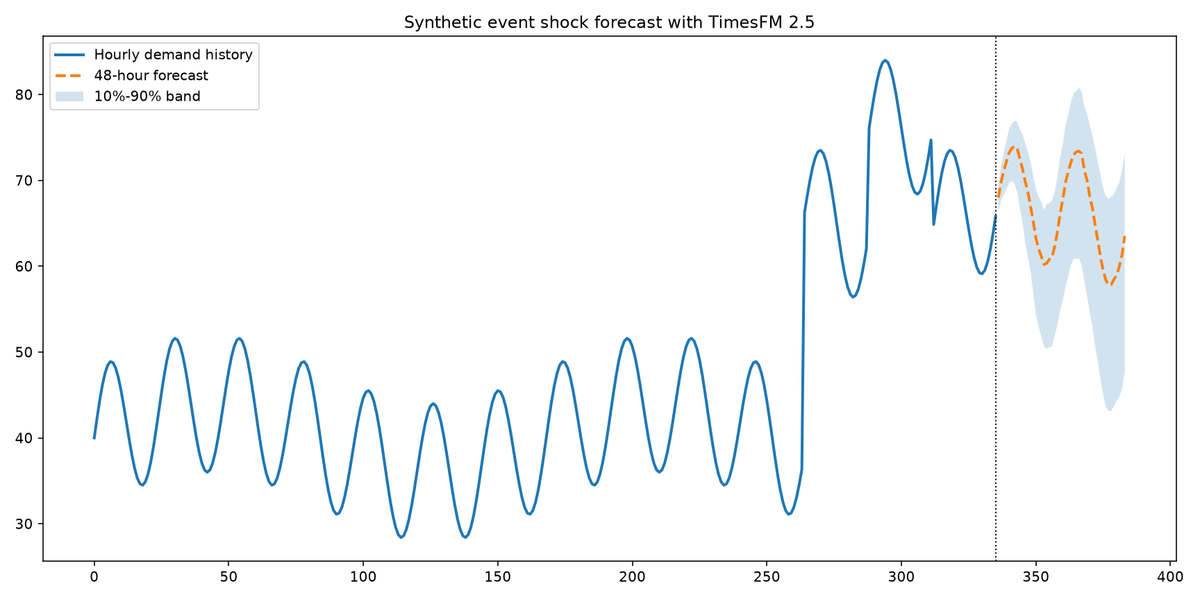
The forecast stays at the elevated level and continues the daily oscillation. Its first p50 value is about 68.16, rather than returning to the baseline near 40. This result makes sense given the input: the elevated period runs all the way to the forecast boundary, and the model receives no information that the event is about to end.
The p10-p90 interval also becomes wider as the forecast horizon increases. That shows increasing predictive dispersion from the model, but it does not tell us why the interval widens or whether the model identified the event as a one-off occurrence.
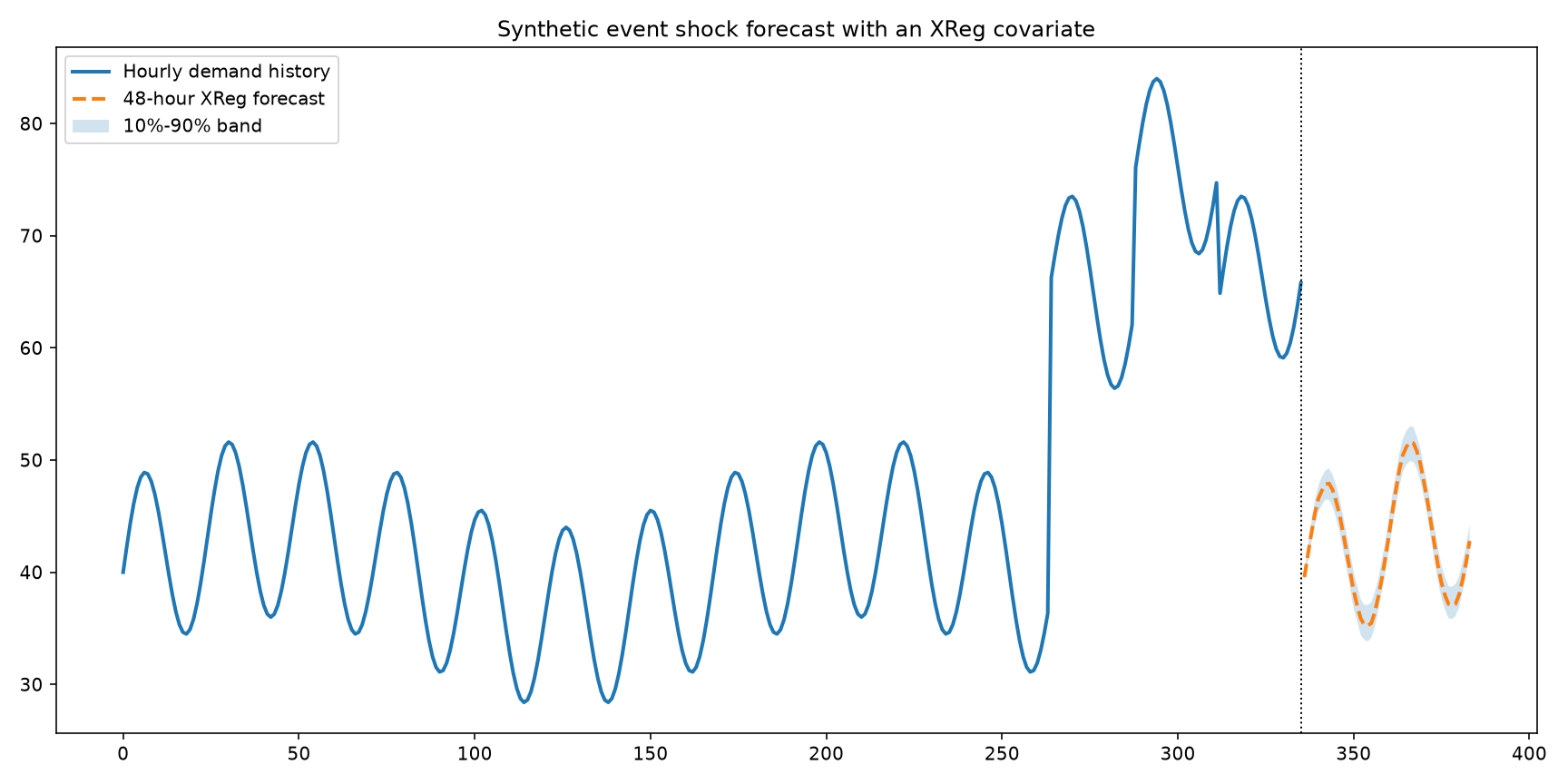
We can give the model more information about the event by adding a past-and-future covariate that indicates whether the event is active. The covariate is a binary array with 1 for the event hours and 0 for normal hours. Unlike TimesFM 2.5's separate linear XReg stage, TimesFM 3.0 consumes this covariate natively during forecasting.
HORIZON = 48


def build_series_and_covariate() -> tuple[np.ndarray, np.ndarray]:
    hours = np.arange(14 * 24)
    daily_cycle = 40 + 8 * np.sin(2 * np.pi * hours / 24)
    weekly_cycle = 4 * np.sin(2 * np.pi * hours / (24 * 7))
    history = daily_cycle + weekly_cycle

    event_active = np.zeros(len(history) + HORIZON, dtype=np.float32)
    event_start = len(history) - 72
    event_active[event_start : len(history)] = 1

    history[event_start : event_start + 72] += 28
    history[event_start + 24 : event_start + 48] += 12
    return history.astype(np.float32), event_active


def main() -> None:
    history, event_active = build_series_and_covariate()
    model = load_model()
    point_forecast, quantile_forecast = forecast_series(
        model,
        history,
        horizon=HORIZON,
        past_future_covariates=event_active,
    )
With the covariate, the model can see that the event ends at the forecast boundary. Its first p50 forecast drops to about 40.09 and then follows the normal daily cycle. The p10-p90 interval is also much narrower than in the forecast without the event schedule.
Walmart weekly sales 
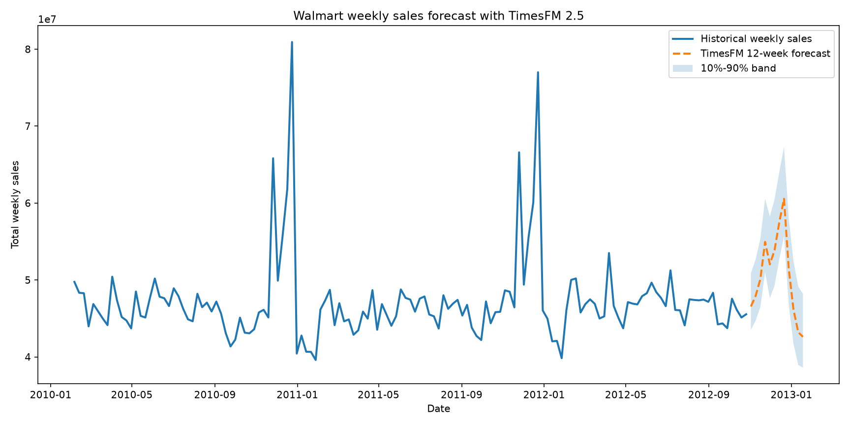
The second example uses the Walmart Recruiting - Store Sales Forecasting dataset. The local train.csv contains 421,570 store-department rows for 143 Fridays between February 2010 and October 2012.
The demo application aggregates all store-department rows in the dataset into one weekly series:
    frame = pd.read_csv(csv_path, usecols=["Date", "Weekly_Sales"])
    frame["Date"] = pd.to_datetime(frame["Date"])
    weekly_sales = frame.groupby("Date")["Weekly_Sales"].sum().sort_index()
Then it loads the model and forecasts the next 12 weeks:
    history = weekly_sales.to_numpy(dtype="float32")
    model = load_model()
    point_forecast, quantile_forecast = forecast_series(
        model, history, horizon=args.horizon
    )
The observed series contains two large year-end peaks. The seasonal component captures these recurring peaks, while the trend changes much more gradually.
TimesFM 3.0 forecasts a p50 increase from about 46.8 million dollars in the first week to 60.0 million for the week ending November 23 and 71.8 million for the week ending December 21. It has recovered the two holiday peaks from the historical sequence without being given calendar labels.
NVIDIA adjusted closes 
In the third example, we forecast the adjusted closing prices of NVIDIA stock. The data is downloaded from Yahoo Finance using the yfinance library. The script selects a rolling two-year window of daily data and uses the adjusted closing prices for forecasting.
    prices = yf.download(
        "NVDA", period="2y", interval="1d", auto_adjust=True, progress=False
    )
    close = prices["Close"]
    if getattr(close, "ndim", 1) != 1:
        close = close.squeeze("columns")

    close_series = close.dropna().to_numpy(dtype="float32")

    if len(close_series) < 200:
        raise RuntimeError("Expected at least 200 closing prices from Yahoo Finance")

    history = close_series[-512:]
The model forecasts 30 trading observations, not 30 calendar days. That usually spans about six calendar weeks.
    model = load_model()
    point_forecast, quantile_forecast = forecast_series(model, history, horizon=30)
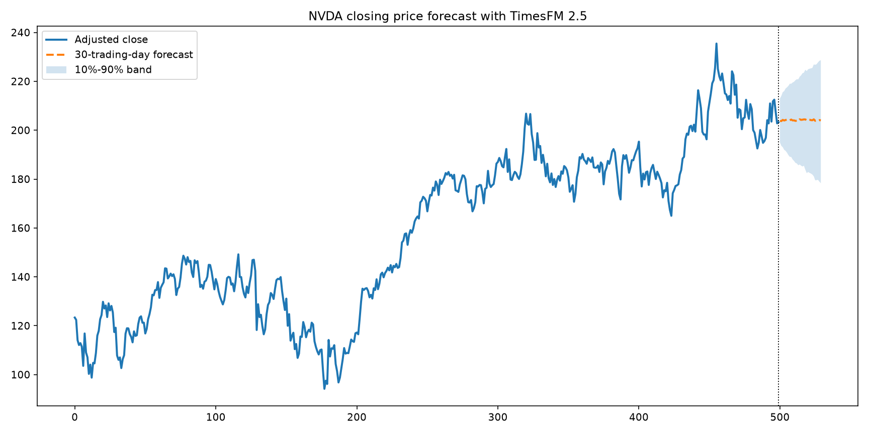
In the run used for this updated chart, the p50 forecast stays nearly flat: it starts at about 224.60 and ends at 226.87. The p10-p90 interval expands from roughly 217.92-231.04 at step one to 205.29-247.90 at step 30. The model sees only the price history; it does not see trading volume, earnings, news, the market calendar, or broader market data. This is a demonstration, not an investment forecast.
German electricity load 
The final example uses the Open Power System Data time-series package, version 2020-10-06. The selected DE_load_actual_entsoe_transparency column contains Germany's total load in MW as published by the ENTSO-E Transparency Platform.
The script downloads the hourly CSV, forward-fills missing values, gives TimesFM the final 28 days as context, and forecasts 168 hours. The chart displays only the last seven days of the input next to the seven-day forecast.
def load_energy_series() -> np.ndarray:
    try:
        frame = pd.read_csv(URL, index_col=0, parse_dates=True)
        return frame[COLUMN].ffill().dropna().to_numpy(dtype="float32")
    except Exception as exc:
        print(f"Warning: TLS-verified download failed ({exc}); retrying with TLS verification disabled.")
        context = ssl._create_unverified_context()
        with urllib.request.urlopen(URL, context=context) as response:
            frame = pd.read_csv(io.BytesIO(response.read()), index_col=0, parse_dates=True)
        return frame[COLUMN].ffill().dropna().to_numpy(dtype="float32")
    load = load_energy_series()

    history = load[-24 * 28 :]
    model = load_model()
    point_forecast, quantile_forecast = forecast_series(
        model, history, horizon=24 * 7
    )
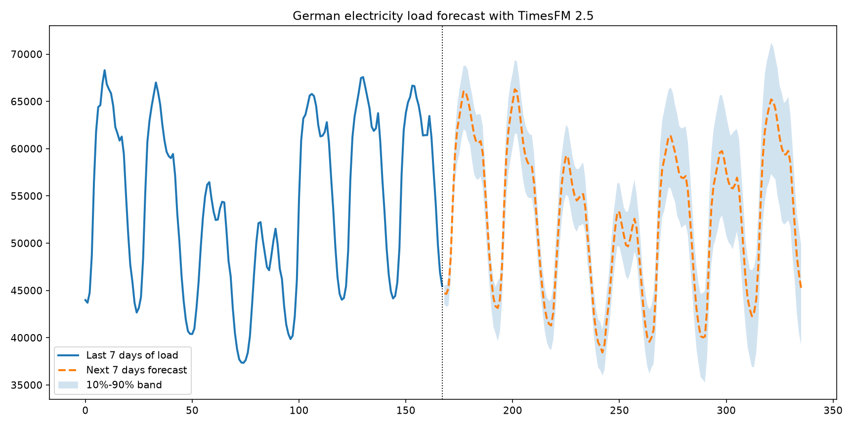
The p50 forecast continues the strong within-day cycle and the differences between weekdays and the weekend visible in the history. The first forecast day rises from about 44.8 GW overnight to about 67.2 GW around the daytime peak. The predictive interval grows over the week but remains structured around the recurring load pattern.
Conclusion 
TimesFM makes it easy to produce a zero-shot baseline for very different time series. The same predict() call works for hourly demand, weekly sales, daily market data, and hourly electricity load.
TimesFM 3.0 also makes multivariate forecasting and covariates first-class inputs. The event example shows why that matters: the target history alone suggests that the elevated regime will continue, while a known future event schedule lets the same model forecast the return to baseline.
As with all forecasting models, the quality of the forecast depends on the quality and quantity of the input data. TimesFM can provide a good starting point for forecasting, but it may not always capture all the nuances of a particular time series. It is important to evaluate the forecasts and consider additional modeling techniques or domain knowledge when necessary.